Tutorial

Set Up

To begin, you need an image that you want to mosaic-ify. You can load it like so:

from skimage.io import imread
image = imread('filepath')

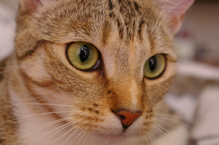
Alternatively, you can use one of the built-in example images provided by scikit-image library. We’ll go with the cat picture, chelsea.

# Load a sample image
from skimage import data
image = data.chelsea()  # cat picture!

Next, you need large collection of images to fill in the tiles in the mosaic. If you don’t have a large collection of images handy, you can generate a collection of solid-color squares. Real photos are more interesting, but solid-color squares are nice for experimentation.

import photomosaic as pm

# Generate a collection of solid-color square images.
pm.rainbow_of_squares('pool/')

# Analyze the collection (the "pool") of images.
pool = pm.make_pool('pool/*.png')

Basic Example

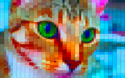
Now we have everything we need to make a mosaic. Specify the target image (image), the pool of available tile images (pool), and the number of tiles to divide the image into.

# Create a mosiac with 30x30 tiles.
mos = pm.basic_mosaic(image, pool, (30, 30))

Now mos is our mosaic. We can save it

from skimage.io import imsave
imsave('mosaic.png', mos)

or plot it using matplotlib.

import matplotlib.pyplot as plt
plt.imshow(mos)

To make a more detailed mosaic, subdivide tiles in important regions. The optional depth parameter selectively splits tiles into quadrants if they contain a certain amount of contrast.

mos = pm.basic_mosaic(image, pool, (30, 30), depth=1)

More fine-grained control over tile partitioning is shown in the next section.

Detailed Example

Prepare the Image

As in the basic example above, we start with a target image, image, and a collection of candidates for the mosaic, pool.

The image (represented in Python as a numpy array) should be specified as floating-point values in the domain 0-1. The utility function img_as_float ensures that that is the case.

# Size the image to be evenly divisible by the tiles.
from skimage import img_as_float
image = img_as_float(image)

Several of the next steps rely on judging the relative similarity of colors. To that end, we convert the colors in image from an RGB (“red green blue”) representation to a perceptually-uniform color space. In this representation, the mathematical difference between two colors is a more accurate estimate of their perceived “difference” to the human vision system.

(In the Set Up above, make_pool() automatically did this for all of the images in the pool before analyzing their colors.)

# Use perceptually uniform colorspace for all analysis.
import photomosaic as pm
converted_img = pm.perceptual(image)

Optional: Optimize the Color Palette

For best results, use adapt_to_pool() to “stretch” the color palette of the image to match the colors available in the pool of candidate images. This greatly improves the contrast in the final result.

# Adapt the color palette of the image to resemble the palette of the pool.
adapted_img = pm.adapt_to_pool(converted_img, pool)

Details and illustrations are given in the section, Palette Adjustment.

Partition Tiles

We will partition the image into tiles. But first, we rescale it (and crop it if necessary) so that it is evenly divisive. As in the basic example above, the grid_dims gives the number of tiles along each dimension and depth (default 0)` gives the number of times a tile may be subdivided.

scaled_img = pm.rescale_commensurate(adapted_img, grid_dims=(30, 30), depth=1)

Now, partition the image into tiles.

tiles = pm.partition(scaled_img, grid_dims=(30, 30), depth=1)

The result is a list of (y, x) slices into the image.

[(slice(0, 32, None), slice(0, 48, None)),
 (slice(0, 32, None), slice(48, 96, None)),
 (slice(0, 32, None), slice(96, 144, None)),
 ...<snip>...
 (slice(288, 320, None), slice(336, 384, None)),
 (slice(288, 320, None), slice(384, 432, None)),
 (slice(288, 320, None), slice(432, 480, None))
]

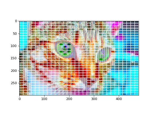
Optionally, visualize the tile layout. (Recall that scaled_img is represented in the perceptually-uniform color space; we have to convert it back to RGB for visualization.)

annotated_img = pm.draw_tile_layout(pm.rgb(scaled_img), tiles)

# Save the result with imsave, or plot with matplotlib:
import matplotlib.pyplot as plt
plt.imshow(annotated_img)

Match Tiles to Pool Images

First, analyze the average color of each tile in the target image.

import numpy

# Reshape the 3D array (height, width, color_channels) into
# a 2D array (num_pixels, color_channels) and average over the pixels.
tile_colors = [numpy.mean(scaled_img[tile].reshape(-1, 3), 0)
               for tile in tiles]

The result is a list of colors, one for each tile in tiles. The values in pool were generated using the same algorithm.

The function simple_matcher takes the analyzed colors in pool and loads them into a data structure for fast nearest-color lookups (a KD tree). It returns a function, match. We map match map onto each tile color to find the corresponding tile’s best match in the pool.

# Match a pool image to each tile.
match = pm.simple_matcher(pool)
matches = [match(tc) for tc in tile_colors]

Note

A different strategy for characterizing the tiles and the pool could be used. The simpler_matcher expects that each tile and each element in the pool is summarized by some vector. Additionally, a more complex matching algorithm — say, one that avoids using any element in the pool more than once — could also be used in place of simple_matcher.

Draw Mosaic

First, create a “canvas” image on which to draw the mosiac. Use numpy functions for generating a “white” or “black” canvas of the right shape,

import numpy
canvas = numpy.ones_like(scaled_img)  # white canvas
canvas = numpy.zeros_like(scaled_img)  # black canvas

or load a background image and scale/crop it the right shape.

from skimage.io import imread
canvas = pm.crop_to_fit(imread('filename'), rescaled_img.shape)

Finally, draw the mosiac.

# Draw the mosaic.
mos = pm.draw_mosaic(canvas, tiles, matches)

Drawing is typically the slowest step. Most of the time is spent resizing images from the pool to fit their assigned tile in the mosaic. To speed up repeated draws, reuse the cache of resized pool images.

cache = {}
mos1 = pm.draw_mosaic(canvas1, tiles1, matches1, resized_copy_cache=cache)
# Now cache is filled with resized copies of any images used in ``mos1``.

# This will be faster:
mos2 = pm.draw_mosaic(canvas2, tiles2, matches2, resized_copy_cache=cache)